Basic Climate Data
New data for Germany and Bavaria
In 2025, there was an UPDATE with the following additions:
- - The climate database has been updated for the observation period up to 2020.
- - The climate model ensemble was supplemented with additional model runs (Euro-Cordex) and expanded to include historical simulations.
- - The bias correction of the simulation data was performed using in-house software.
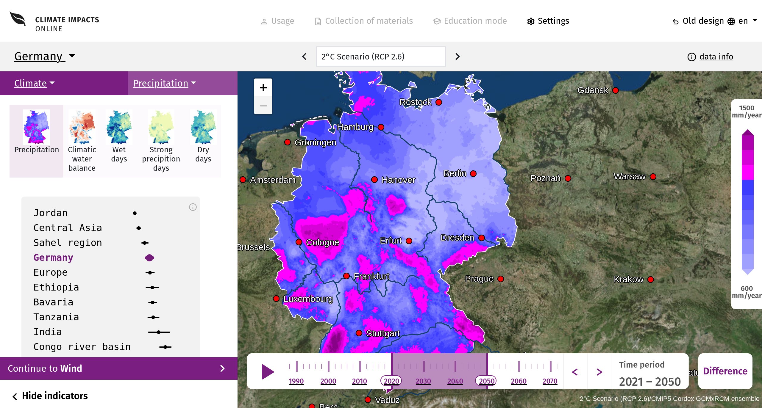
- - The result data was interpolated onto a finer grid, taking topographical features into account.
Differences
The difference to the Impact2C dataset used from 2019 onwards is essentially a more comprehensive model ensemble of 17 runs for the RCP8.5 scenario. The resulting statistics for selected climate indicators for a 30-year period are therefore based on 30x17=510 annual values (instead of 120). In comparison, there may be significant deviations in the development of individual indicators.
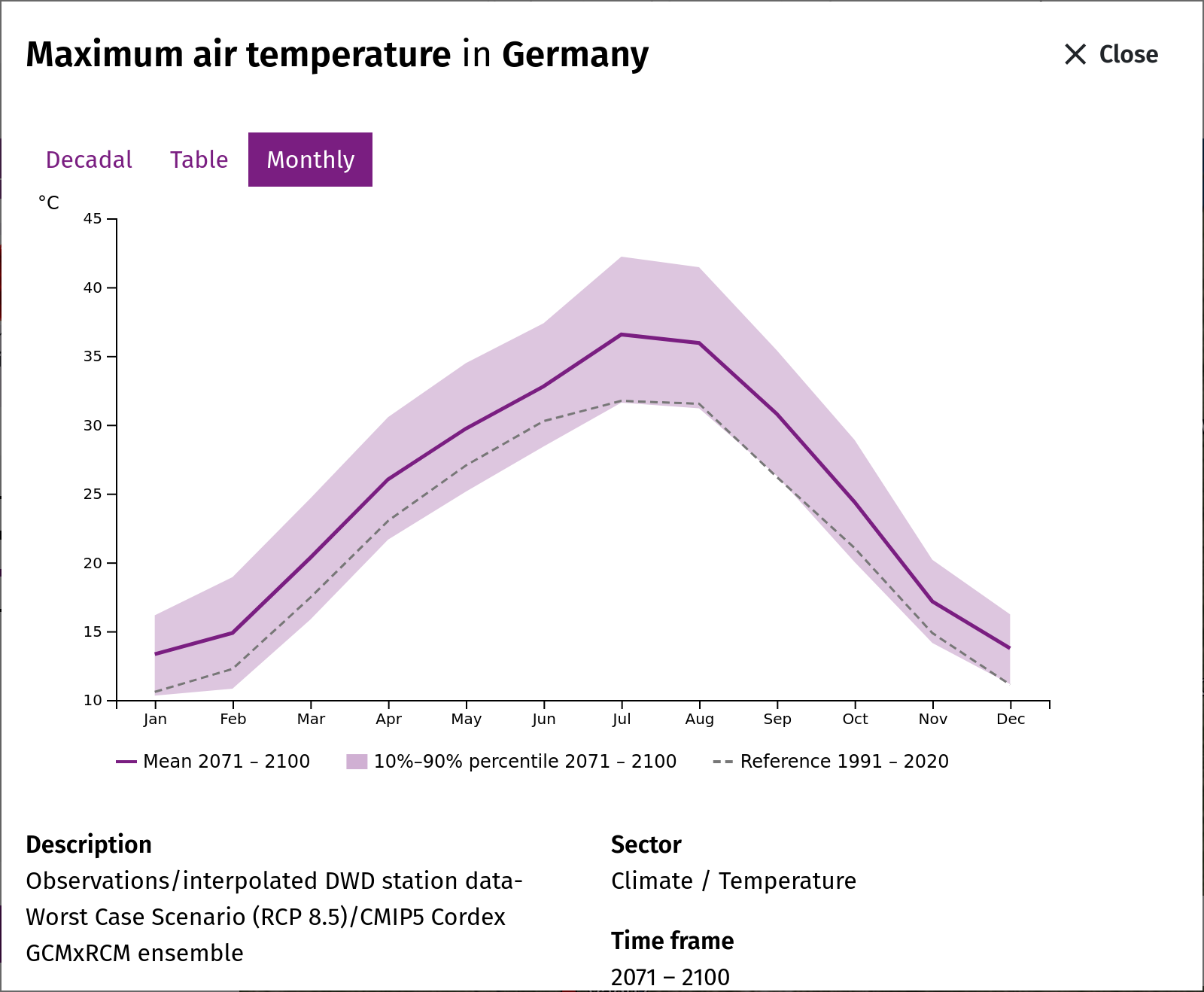
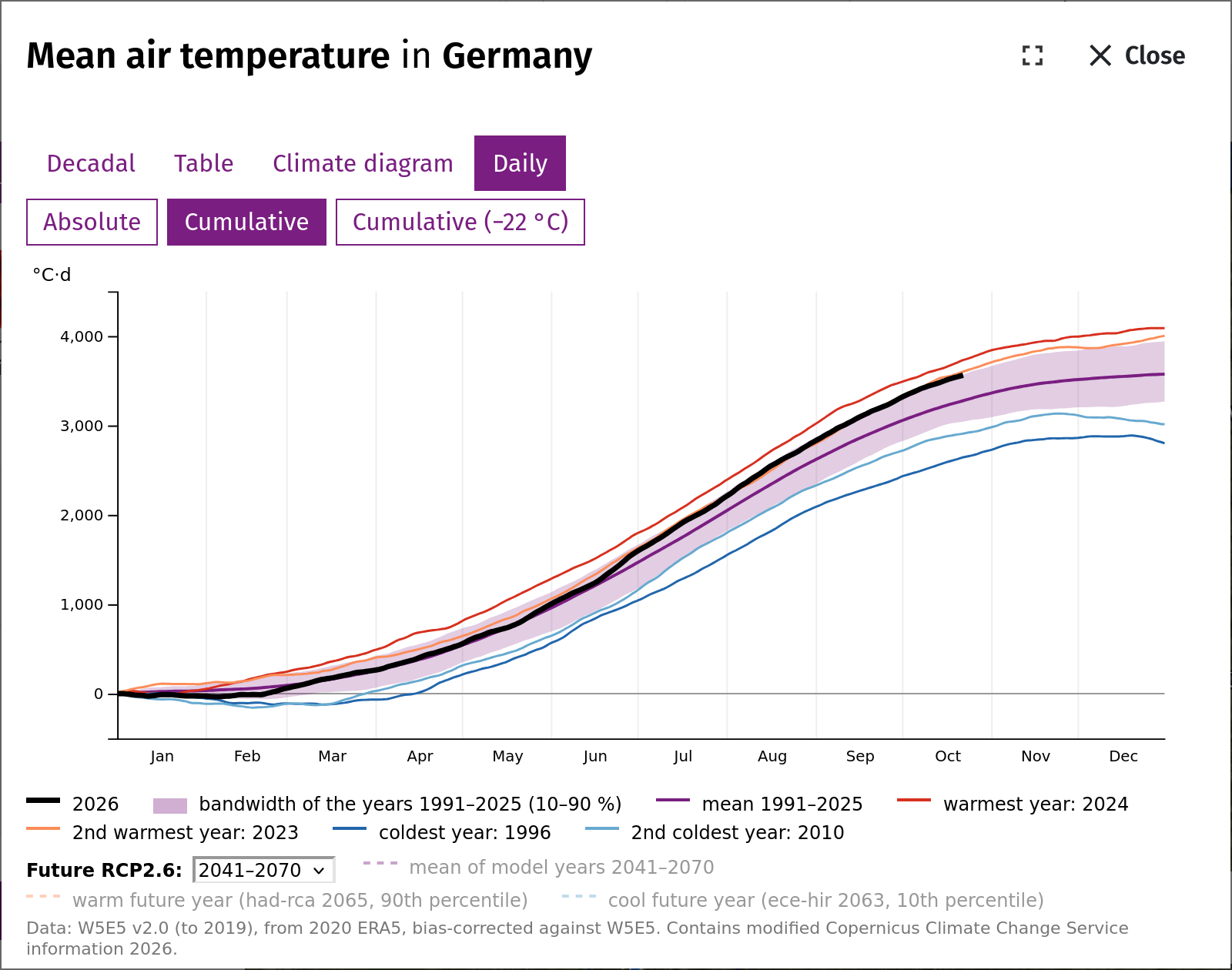
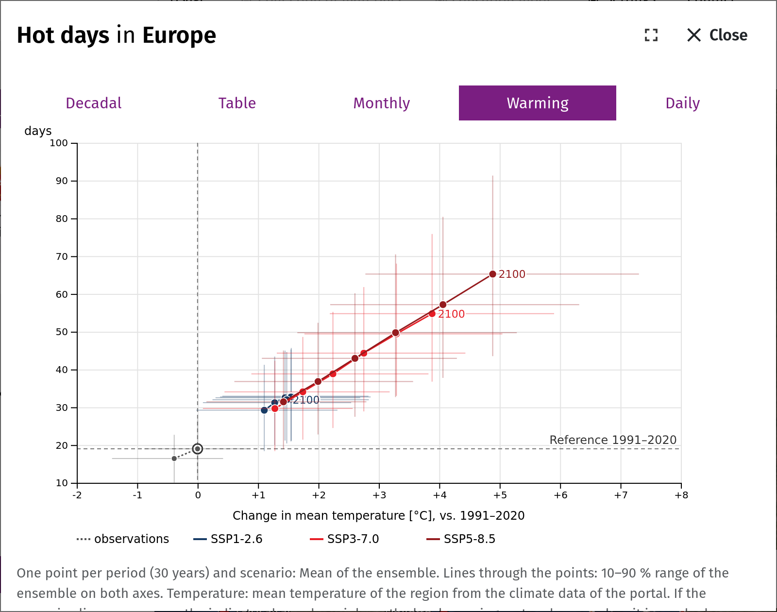
The range of the annual mean temperature in Germany remains roughly the same at 11°C to 14°C (RCP8.5 to 2100). Greater differences are apparent in the mean number of hot days. In the current data, the value is just under 30 days. Previously, it was slightly more than 20 days in Germany.
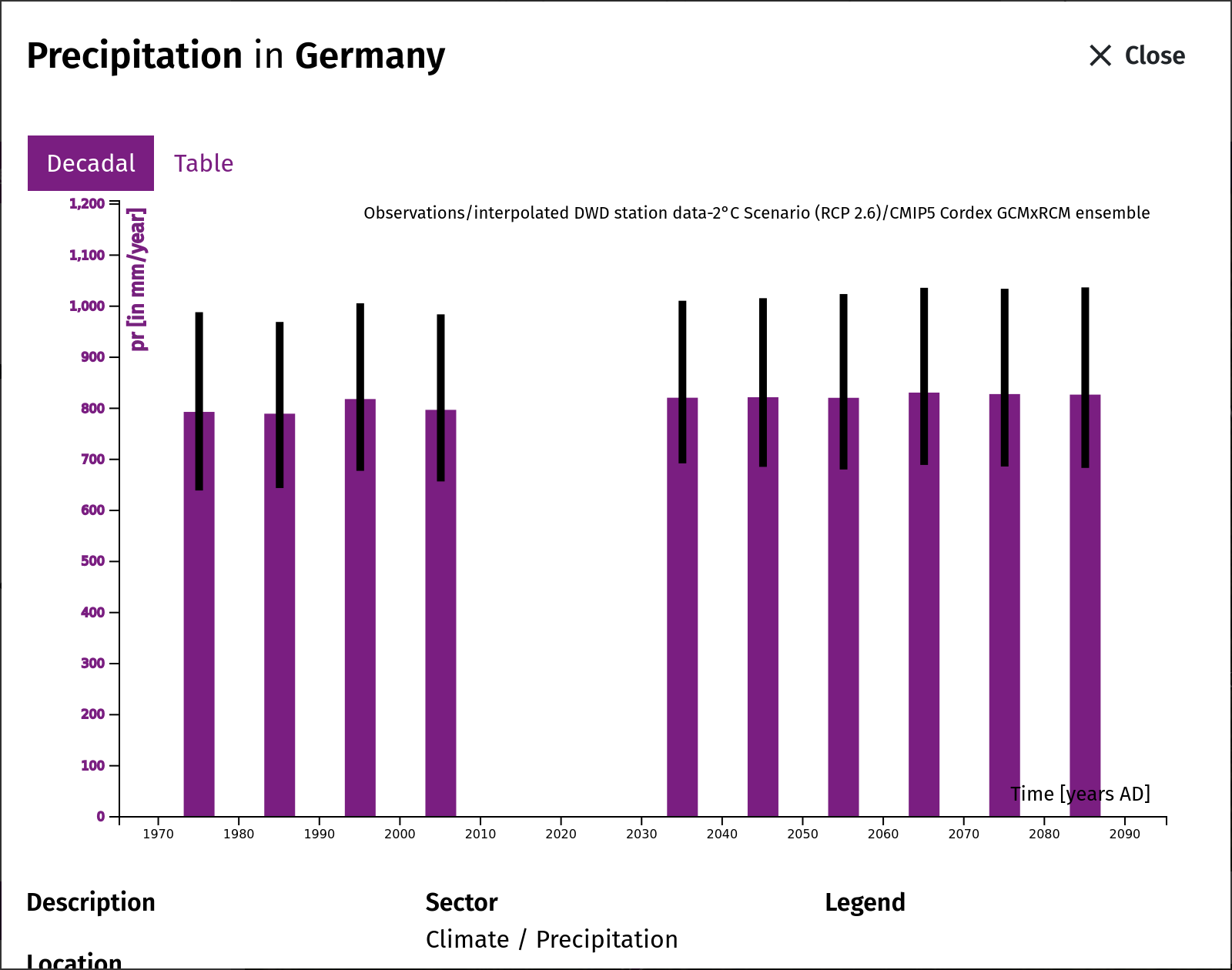
The more comprehensive ensemble also has an impact on total precipitation. The more models there are, the greater the range of variability in annual precipitation. On average, developments remain at historical levels. However, more heavy rainfall and higher average temperatures favor longer dry spells.
Observation data: 1961-2020
Only measuring stations that have been part of the DWD station network since 1961 were taken into account for updating the observation data set. These include approximately 220 synoptic stations and approximately 1,200 precipitation stations. All of them provide daily values for meteorological parameters. Due to the limited station density, small-scale phenomena and regional characteristics in particular cannot be depicted with complete accuracy. This station network also forms the basis for the preparation of scenario data (see Interpolation).
Climate model ensemble: historical and future
The RCP8.5 climate model ensemble, which currently comprises 17 simulations, has been supplemented with historical simulation periods dating back to 1971. The entire simulation period thus covers a total of 130 years. The ensemble for the RCP2.6 scenario is significantly smaller because fewer runs are available for it. For the historical period, the current version allows comparisons between developments in the model ensemble and in the observations. Many of the indicators show that the simulations are consistent with the observations. Phenomena such as spring droughts show discrepancies that indicate weaknesses in the model.
Climate model ensemble
Regional climate model ensemble
In order to derive regional climate impacts from future climate development paths (in accordance with the RCP scenarios), it is necessary to refine global climate model simulations (GCMs) for large regions such as Europe. This is usually achieved by using them as input for higher-resolution regional climate models (RCMs). These models are able to reproduce the regional characteristics of temperature and precipitation distribution more realistically, as they better reflect effects caused by topography and land use, among other things.
Extensive simulation data from [Euro-Cordex] https://cds.climate.copernicus.eu/datasets/projections-cordex-domains-single-levels?tab=download provides the basis and data foundation (see table) for enabling climate services for Europe, Germany, and federal states. The simulation period covers the historical periods from 1971 onwards and extends into the scenario period until 2100. Each individual model combination represents a possible realization of climatic and meteorological development. Typically, time slices of 30 years are considered, whose variability and means are explained by 30x17=510 annual values. The totality of the values results in ranges that are composed of both internal variability and model uncertainty.
It is well known that there are systematic errors between models and measurements. For the historical comparison period, these can be quantified in order to adjust (align) the simulation values. Existing trends in the data are retained in the process. There are established methods for this in climate impact research (Lange, 2019). This is because the size of the so-called model bias is not the sole criterion for evaluating climate model simulations.
Daily data on a uniform grid is required to align the model values with the observation values. This is specified by the generated observation data set. To transfer the model values to the observation grid, the model data is first transferred to the station network. To do this, the values of the nearest grid point are assigned to the station coordinates. Interpolation is then performed in the same way as for the base data set. This step ensures that simulation data and observation data have the same spatial assignment. In this way, climatic developments can be seamlessly represented in map and diagram form.
The two climate model ensembles RCP2.6 and RCP8.5 span the possible range of events within which the future climate in Germany may develop. Existing discrepancies between observed and simulated developments cannot be resolved at this point in time, as this is a continuous process of further developing scientific knowledge. Phenomena that trigger prolonged drought are therefore the subject of current research with relevance across sectors of climate impact research.
| GCM/RCM | CLMcom CCLM4-8-17 | SMHI RCA4 | KNMI RACMO22E | DMI HIRHAM5 |
| MPI-M MPI-ESM-LR | RCP8.5 | RCP8.5/2.6 | ||
| CNRM-CERFACS CNRM-CM5 | RCP8.5 | RCP8.5 | RCP8.5 | RCP8.5 |
| MOHC HadGEM2-ES | RCP8.5 | RCP8.5/2.6 | RCP8.5/2.6 | RCP8.5 |
| IPSL IPSL-CM5A-MR | RCP8.5 | |||
| ICHEC EC-EARTH | RCP8.5/2.6 (r12) | RCP8.5/2.6 (r12) | RCP8.5 (r1) RCP2.6 (r12) | RCP8.5 (r1) RCP2.6 (r3) |
| NCC NorESM1-M | RCP8.5 | RCP8.5 |
Table: Simulation matrix of the underlying combinations of regionalized global model simulations (GCMs) by regional models (RCMs): RCP8.5 – 17 models, RCP2.6 – 7 models. No EuroCordex simulations are available for the RCP scenarios for the empty fields. In brackets: ensemble member (realisation) of EC-EARTH used.
Further Literature: Lange, S.: Trend-preserving bias adjustment and statistical downscaling with ISIMIP3BASD (v1.0), Geosci. Model Dev., 12, 3055–3070, https://doi.org/10.5194/gmd-12-3055-2019, 2019.
Bandwidth
The underlying regional climate model ensemble includes seven simulations for the RCP 2.6 scenario and 17 simulations for the RCP 8.5 scenario.
To estimate the ranges, model uncertainty and internal (year-on-year) variability were combined, sorted, and the value below which 10% and 90% of the values lie was used for the time series representation. Only the mean values are shown on the map. For a 30-year period and a model ensemble of 17 simulations, this means a pool of 17 x 30 = 510 annual values is available for the respective climate indicators.
Note: During the observation period, the range results exclusively from the internal variability of 30 annual values. Against this background, model uncertainty and internal variability were combined to estimate the range in the scenario data.
Interpolation
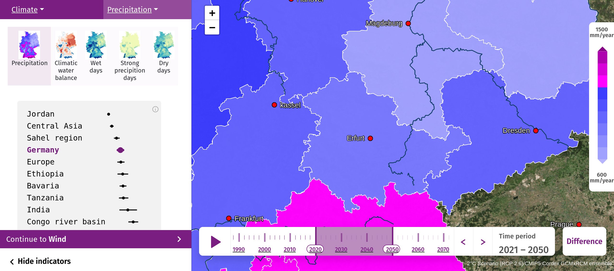
To display the climate indicators derived from the daily climate data, a method was used in which the available information at the locations of the measuring stations was interpolated to grid points. Their spatial resolution is approximately 4 x 4 km, for which elevation values from a digital terrain model are also available. Among other things, the method takes into account existing gradients of values at different altitudes in the station network. Before the actual interpolation, the altitude effects in the station network are eliminated. The value sought at the corresponding grid point is then determined by a weighted summation of the station data within a specified radius of influence (neighboring stations), whereby the sum is then divided by the number of stations. The elevation effect is then applied to the target grid according to the elevation values.
Global radiation (rsds): A different method is used for global radiation. A test in which each station was left out in turn and predicted from the others showed that the elevation correction worsens the results here. The values are therefore interpolated without an elevation gradient, using radial basis functions of the distance in kilometres, complemented by a constant and a linear term. This lowers the mean error at the stations from about 20 to about 16.5 W/m2; values outside 0–400 W/m2 are capped. The observed global radiation itself is derived from the sunshine duration at the stations (see the explanation of the variable).
Further Literature:
Cressie N., 1993, Statistics for spatial data, Wiley Series in Probability and Statistics
https://app.readthedocs.org/projects/pykrige/downloads/pdf/latest/
Observation data
Historical observations of climatic developments, as presented in the Climate section, are based on station data that has been part of the DWD measurement network since 1961.
They provide daily values for meteorological parameters at approximately 220 synoptic stations and approximately 1,200 precipitation stations.
This station data set forms the basis for homogenization and spatial interpolation to a high-resolution grid, taking topographical conditions into account. Values from neighboring stations are taken into account during homogenization and interpolation. Derived climate indicators are calculated on the basis of the interpolated daily data. Possible artifacts cannot be ruled out in individual cases.
Scenario Selection
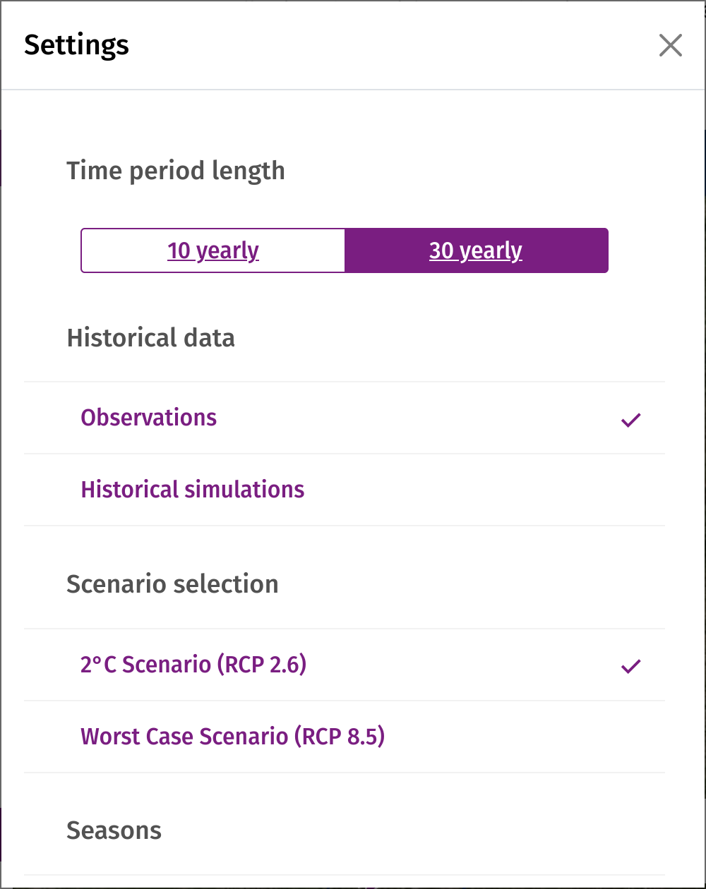
The KlimafolgenOnline portal shows two of the four Main Representative Concentration Pathways (RCP2.6, RCP4.5, RCP6.0 and RCP8.5). These were developed by the scientific community for the fifth assessment report of the Intergovernmental Panel on Climate Change (IPCC).
The RCP scenarios 2.6 and 8.5 used in the portal take into account different levels of greenhouse gas-induced radiative forcing for the period 2021-2100. The decisive factor for the respective differences in temperature increase in the scenarios is the intensity of future climate protection measures from 2021 to 2100, which influence radiative forcing and greenhouse gas concentrations.
The RCP 2.6 scenario shows a possible development that is expected to comply with the global two-degree limit. This requires strong climate protection measures. The two-degree limit is a political target, as scientists believe that the effects of climate change would remain manageable if warming were to remain below this temperature. More detailed information can be found in the German synthesis report of the IPCC's Fifth Assessment Report. This document is available as a PDF file in the menu under Climate Knowledge. At the UN Climate Change Conference in Paris in December 2015, 195 countries agreed on a new agreement to combat global warming. According to this agreement, global warming is to be limited to “well below two degrees” compared to pre-industrial conditions.
The RCP 8.5 scenario is the worst-case scenario. It describes a possible climate development with continuously rising greenhouse gas emissions and no additional climate protection measures. Based on the scenario runs of the global climate models currently available, this results in a global mean temperature increase of between 3.6 °C and 4.1 °C by 2100 compared with pre-industrial levels.
In Germany, the average temperature increase by 2100 compared to pre-industrial levels will be in the range of +2°C (RCP2.6) and +5°C (RCP8.5).
Crop yields in Germany: the statistical model ABSOLUT
How the model works and how it is used for Germany
The yields of winter wheat and silage maize are calculated with ABSOLUT v1.2 (Conradt 2022), a statistical model developed at PIK. ABSOLUT does not simulate plant growth. For each district it determines from observations how the yield of a year depended on the weather of that year. For this it uses multiple linear regressions on monthly values of temperature, precipitation and solar radiation. For every district it selects up to four combinations of a span of months and one of these variables that explain the observed yields best. The models were fitted on the district yield statistics 1991–2021 (Duden et al. 2024).
An example: in the district of Augsburg the winter wheat yield depends mainly on the temperature in May and June; every degree warmer lowers it by about 3 dt/ha. In addition, the model uses the temperature in January and February and the solar radiation in May and June and from November to January. For silage maize it is mainly the temperature from June to August (about −21 dt/ha per degree) and the precipitation in July and August (about +1.5 dt/ha per 10 mm more per month).
For the projections, the regressions are driven by the climate simulations of the portal (EURO-CORDEX: 17 model runs for RCP8.5, 7 for RCP2.6). The yield of a future year is the observed mean yield of 1991–2020 in that district plus the climate effect of the weather of that year relative to 1991–2020 in the same simulation. This keeps the level of the observed yields: in 1991–2020 the modelled district means deviate from the observed means by at most about 1 %.
Model limits
- Technology and management are kept constant. The upward trend of the past (varieties, fertiliser, management) is not continued. The results show only the effect of the climate.
- No CO₂ effect. Higher CO₂ concentrations can raise yields, mainly of wheat; this is not included.
- Drought years are underestimated. For 2018 the model gives −7 % for winter wheat in Germany (observed −10 %) and −21 % for silage maize (observed −26 %). The projected losses are therefore rather a lower estimate.
- Beyond experience. After about 2050 the simulated climate increasingly lies outside the range the models were fitted on. The climate effect is therefore bounded to ±50 % of the mean yield.
Which districts are shown
A district is shown only if its model passed an independent test. The model had to predict the change of the yield from one year to the next for years it had not seen when it was built, and do so at least as well as the simple assumption of the same average change every year (Nash–Sutcliffe efficiency ≥ 0). This applies to 270 of 353 districts for winter wheat and 301 of 331 for silage maize. A federal state is shown if such districts make up at least half of its area. This is not the case for winter wheat in North Rhine-Westphalia and Saarland, and for silage maize in Rhineland-Palatinate. City states without yield statistics are left blank.
Results for Germany
Mean of the districts shown; the percentage is the change of the ensemble median compared with 1991–2020; in brackets the spread of the model ensemble (10th to 90th percentile).
| Winter wheat | Silage maize | |
|---|---|---|
| 1991–2020 | 69.6 dt/ha (61–78) | 427 dt/ha (370–484) |
| RCP2.6, 2071–2100 | 68.3 dt/ha, −2 % | 418 dt/ha, −2 % |
| RCP8.5, 2031–2060 | 67.1 dt/ha, −3.5 % | 412 dt/ha, −3.5 % |
| RCP8.5, 2071–2100 | 63.2 dt/ha, −9 % (54–72) | 378 dt/ha, −11.5 % (316–440) |
With strong climate protection (RCP2.6) the yields of both crops remain almost unchanged. With high emissions (RCP8.5) they decrease slowly until the middle of the century and markedly afterwards, by about one tenth by the end of the century. Silage maize loses somewhat more than winter wheat; a plausible reason is that maize grows through the whole summer, whereas wheat is harvested in July (not evaluated in the models). The spread between the model runs is of the same order as the change itself, so single years and single districts can deviate considerably.
Reference
Conradt, T. (2022): Choosing multiple linear regressions for weather-based crop yield prediction with ABSOLUT v1.2 applied to the districts of Germany. International Journal of Biometeorology 66, 2287–2300. doi:10.1007/s00484-022-02356-5
Duden, C., Nacke, C., Offermann, F. (2024): German yield and area data for 11 crops from 1979 to 2021 at a harmonized spatial resolution of 397 districts. Scientific Data 11, 95. doi:10.1038/s41597-024-02951-8 (dataset: doi:10.3220/DATA20231117103252-0)
Viticulture models: phenology, late frost, harvest and grape berry moth
The viticulture indicators for Germany apply to the grape variety Riesling on level ground. They are computed for every grid point (about 1 km) from daily weather data – for the observations since 1961 and for all 24 climate model runs of the scenarios RCP2.6 and RCP8.5. They are shown only where the Huglin index, averaged over the model ensemble and the period, reaches at least 1500; below that, viticulture is thermally not recommended (Stock et al. 2007). These areas are grey on the map.
Bud break and start of flowering: the phenology model
Bud break and start of flowering are computed with the phenology model of Hoppmann & Berkelmann-Löhnertz (2000), developed for Riesling in Geisenheim and applied to Germany in PIK Report 106 (Stock et al. 2007). It adds up a temperature-dependent development rate; when the sum reaches a threshold, the stage is reached. We use the Python version by C. Menz; it reproduces the Fortran version by Th. Kartschall within about one day.
With the original Geisenheim thresholds, bud break at the stations of the phenology network of the German Weather Service (169 Riesling stations, 1991–2024) came 4–5 days late on average. The thresholds were therefore refitted to this network. The check used stations not involved in the fit and a period not used (fit 1991–2007, test 2008–2024 and the other way round): the mean error is below 2.5 days, in a single year about 6 days, and the trend is reproduced. Start of ripening and harvest ripeness of the model are not used: they scatter by about 14 days from station to station, and harvest ripeness came 14 days late on average.
Late frost
Counted are years with at least one day below 0 °C (minimum temperature at 2 m) from the 10th day after bud break to the day before flowering. This window was chosen because it matches the yield losses best in a comparison with the wine-must yields of the wine regions (statistical offices of Rhineland-Palatinate and Germany, 2000–2024). At the weather stations the computed late frost agrees with the one from the station data in 98 % of the station-years. Radiation frost in clear, calm nights (minimum temperature 0 to 2.5 °C) is not included: the rule for it flags about 40 % of the years even at stations, shows no relation to the yields, and the climate models underestimate the wind.
Harvest date
The typical date of the main harvest is the day on which the sum of daily mean temperatures from 1 April (limited to 0 to 25 °C) reaches 2980 °C days (after Parker et al. 2020). The threshold was fitted to the harvest dates of the DWD network (2,116 station-years): mean deviation 11 days, trend 1991–2024 as observed (3.5 days per decade earlier).
Grape berry moth (expert mode)
The start of the 1st and 2nd flight of the European grape berry moth follows the temperature sums of the warning services (1st flight: daily maxima above 0 °C from 1 March, 620 °C days; 2nd flight: daily means above 8 °C from 1 January, 650 °C days). Both reproduce the PIK population model at 15 wine-growing stations within 3–4 days. Whether a 3rd generation forms is decided by the day length during the egg and early larval stage of the 2nd generation: with short days the larvae enter winter rest (diapause). Because the critical day length for Germany is not known precisely, there are two variants: a threshold rule (15.7 hours) and a gradual rule after Baumgärtner et al. (2012). The threshold rule matches the experience that a partial 3rd generation occurs only in warm years; the gradual rule gives considerably more. Observed flight series to check them are not yet available; the grape berry moth indicators are therefore shown in expert mode only.
Limits
All values apply to Riesling on level ground and to the air temperature at 2 m on a grid of about 1 km. Slopes, cold-air sinks, clones, other varieties and management can differ by several days, or clearly in the frost risk.
References
Baumgärtner, J., Gutierrez, A.P., Pesolillo, S., Severini, M. (2012): A model for the overwintering process of European grapevine moth Lobesia botrana populations. Journal of Entomological and Acarological Research 44, e2.
Hoppmann, D., Berkelmann-Löhnertz, B. (2000): The prognosis of phenological stages of Vitis vinifera (cv. Riesling) for optimizing pest management. EPPO Bulletin 30, 121–126.
Parker, A.K. et al. (2020): Temperature-based grapevine sugar ripeness modelling for a wide range of Vitis vinifera L. cultivars. Agricultural and Forest Meteorology 285–286, 107902.
Roditakis, N.E., Karandinos, M.G. (2001): Effects of photoperiod and temperature on pupal diapause induction of grape berry moth Lobesia botrana. Physiological Entomology 26, 329–340.
Stock, M. et al. (2007): Perspektiven der Klimaänderung bis 2050 für den Weinbau in Deutschland (Klima 2050). PIK Report 106.
Deutscher Wetterdienst (DWD), Climate Data Center: phenological observations of the grapevine and daily station data, CC BY 4.0.